


Lab 2 — locality in a GPU
Out: 9/21/2016 Due:Parts 1 and 2 on 10/04/2016, Part 3 on 10/14/2016
Note: Part 2(b) is optional, for extra credit
This lab graciously provided by Kayvon Fatahalian of CMU; originally developed for Kayvon’s course. Do not share material from this lab outside of class.
Overview
In this assignment you will write a parallel renderer in CUDA that draws colored circles. While this renderer is very simple, parallelizing the renderer will require you to design and implement data structures that can be efficiently constructed and manipulated in parallel. This is a challenging assignment so you are advised to start early. Seriously, you are advised to start early. Good luck!
Environment Setup
TACC Stampede Machine
This assignment requires a GPU with CUDA compute capability. We suggest that you use Stampede at TACC.
For general information about using Stampede, please refer to the following links.
https://portal.tacc.utexas.edu/user-guides/stampede#gpu
https://portal.tacc.utexas.edu/user-guides/stampede#running
To start using CUDA on the machine you will need to do the following
- $> module load cuda
CUDA related tools are located in the following path
/opt/apps/cuda/6.5/
You can test sample CUDA codes by copying sample codes to your local directory.
- $> cp -r /opt/apps/cuda/6.5/samples ./
Make sure the CUDA_PATH variable is set properly in the Makefile of any code you are trying to compile. It should be: CUDA_PATH ?= /opt/apps/cuda/6.5/
CUDA
The CUDA C programmer’s guide is an excellent reference for learning how to program in CUDA.
http://docs.nvidia.com/cuda/pdf/CUDA_C_Programming_Guide.pdf
The latest CUDA manual is 7.5 but we will use 6.5.
You can also learn by looking at the sample code that NVIDIA provided.
/opt/apps/cuda/6.5/samples
There are also many tutorials and courses online. For example, this course on Udacity: https://www.udacity.com/wiki/cs344.
Building and Running Starter Code
Download tar ball file and copy it to your account. The file is uploaded on Canvas. Download starter.tgz from here
If you would like to build the starter code, just go into each directory and type ‘make.’ If you want to execute the CUDA application, type the following.
stampede ~/somedirectory/saxpy$> sbatch saxpy.sbatch
Before you submit the job, please modify email address in saxpy.sbatch file and also other *.sbatch files.
There are mainly two queues that can be used for GPU applications.
 gpu
 gpudev
gpudev queue is used for development and usually there is strict limit on how long you can execute. The following is the example of sbatch job submission file.
 #!/bin/bash
 #SBATCH -J saxpy           # job name
 #SBATCH -o saxpy.oj expands to  jobID)
 #SBATCH -n 1              # total number of mpi tasks requested
 #SBATCH -p gpudev     # queue (partition) — normal, development, etc.
 #SBATCH -t 01:30:00        # run time (hh:mm:ss) - 1.5 hours
 #SBATCH —mail-user=someemailaddrofyours@gmail.com
 #SBATCH —mail-type=begin  # email me when the job starts
 #SBATCH —mail-type=end    # email me when the job finishes
 #SBATCH -A Fa16EE382N-20
 ./cudaSaxpy             # run the MPI executable named a.out
Part 1: CUDA Warm-Up 1: SAXPY
To gain a bit of practice writing CUDA programs your warm-up task is to implement the SAXPY function in CUDA. Starter code for this part of the assignment is located in the /saxpy directory of the assignment tarball.
Please complete the implementation of SAXPY in the function saxpyCuda in saxpy.cu. You will need to allocate device global memory arrays and copy the contents of the host input arrays X, Y, and result into CUDA device memory prior to performing the computation. After the CUDA computation is complete, the result must be copied back into host memory. Please see the definition of cudaMemcpy function in Section 3.2.2 of the Programmer’s Guide.
As part of your implementation, add timers around the CUDA kernel invocation in saxpyCuda. Your additional timing measurement should not include the time to transfer data to and from device memory (just the time to execute the computation). Note that CUDA kernel’s execution on the GPU is asynchronous with the main application thread running on the CPU. Therefore, you will want to place a call to cudaThreadSynchronize following the kernel call to wait for completion of all CUDA work. This call to cudaThreadSynchronize should return before stopping the timer.
Question 1. What performance do you observe compared to the sequential CPU-based implementation of SAXPY? Compare and explain the difference between the results provided by two sets of timers (the timer you added and the timer that was already in the provided starter code). Are the bandwidth values observed roughly consistent with the reported bandwidths available to the different components of the machine? (Hint: You should use the web to track down the memory bandwidth of an NVIDIA K20 GPU, and the maximum transfer speed of the computer’s PCIe-x16 bus)
Part 2(a): CUDA Warm-Up 2: Parallel Prefix-Sum
Now that you’re familiar with the basic structure and layout of CUDA programs, as a second exercise you are asked to come up with parallel implementation of the function find_repeats which, given a list of integers A, returns a list of all indices i for which A[i] == A[i+1].
For example, given the array {1,2,2,1,1,1,3,5,3,3}, your program should output the array {1,3,4,8}.
Exclusive Prefix Sum
We want you to implement find_repeats by first implementing parallel exclusive prefix-sum operation.
Exclusive prefix sum takes an array A and produces a new array output that has, at each index i, the sum of all elements up to but not including A[i]. For example, given the array A={1,4,6,8,2}, the output of exclusive prefix sum output={0,1,5,11,19}.
A recursive implementation can be implemented as following. Please read the following if you are not familiar with the topic. http://www.cs.cmu.edu/~15210/lectures/seq-notes.pdf
- void exclusive_scan_recursive(int* start, int* end, int* output, int* scratch)
- {
- int N = end - start;
- if (N == 0) return;
- else if (N == 1)
- {
- output[0] = 0;
- return;
- }
- // sum pairs in parallel.
- for (int i = 0; i < N/2; i++)
- output[i] = start[2*i] + start[2*i+1];
- // prefix sum on the compacted array.
- exclusive_scan_recursive(output, output + N/2, scratch, scratch + (N/2));
- // finally, update the odd values in parallel.
- for (int i = 0; i < N; i++)
- {
- output[i] = scratch[i/2];
- if (i % 2)
- output[i] += start[i-1];
- }
- }
While the above code expresses our intent well, it is not particularly amenable to a CUDA implementation. Therefore, we can unwind the recursion tree and express our algorithm in an iterative manner. The following code should show you how one traverses the recursion tree and unwind it. Luckily for us we do not actually even need a stack to express our code.
The following “C-like” code is an iterative version of scan. We use parallel_for to indicate potentially parallel loops.
- void exclusive_scan_iterative(int* start, int* end, int* output)
- {
- int N = end - start;
- memmove(output, start, N*sizeof(int));
- // upsweep phase.
- for (int twod = 1; twod < N; twod*=2)
- {
- int twod1 = twod*2;
- parallel_for (int i = 0; i < N; i += twod1)
- {
- output[i+twod1-1] += output[i+twod-1];
- }
- }
- output[N-1] = 0;
- // downsweep phase.
- for (int twod = N/2; twod >= 1; twod /= 2)
- {
- int twod1 = twod*2;
- parallel_for (int i = 0; i < N; i += twod1)
- {
- int t = output[i+twod-1];
- output[i+twod-1] = output[i+twod1-1];
- output[i+twod1-1] += t; // change twod1 to twod to reverse prefix sum.
- }
- }
- }
You are welcome to use this general algorithm to implement a version of parallel prefix sum in CUDA. You must implement exclusive_scan function in scan/scan.cu. Your implementation will consist of both host and device code. The implementation will require multiple kernel launches.
Note: The reference scan implemenation above assumes that the input array’s length (N) is a power of 2. In the cudaScan function, we solve this problem by rounding the input array length to the next power of 2 when allocating the corresponding buffers on the GPU. However, we only copy back N elements from the GPU buffer back to the CPU buffer. This fact should simplify your CUDA implementation.
Implementing “Find Repeats” Using Prefix Sum
Once you have written exclusive_scan, you should implement the function find_repeats in scan/scan.cu. This will involve writing more device code, in addition to one or more calls to exclusive_scan. Your code should write the list of repeated elements into the provided output pointer (in device memory), and then return the size of the output list.
When using your exclusive_scan implementation, remember that the contents of the start array are copied over to the output array. Also, the arrays passed to exclusive_scan are assumed to be in device memory.
Grading: We will test your code for correctness and performance on random input arrays.
For reference, a scan score table is provided below, showing the performance of a simple CUDA implementation on a stampede cluster with a K20. To check the correctness and performance score of your scan and find_repeats implementation, run make check_scan and make check_find_repeats respectively. To run on a stampede node, run sbatch scan.sbatch and it will run both checks. Doing so will produce a reference table like so; your score is based solely on the performance of your code. In order to get good credit, your code must perform much better than the provided reference solution.
 -------------------------
 Scan Score Table:
 -------------------------
 ------------------------------------------------------------------------- ------------------
 | Element Count   | Serial Time     | Fast Time       | Your Time       | Score           |
 -------------------------------------------------------------------------------------------
 | 10000           | 0.036           | 0.512           | 0.012 (F)       | 0               |
 | 100000          | 0.382           | 0.862           | 0.071 (F)       | 0               |
 | 1000000         | 3.837           | 1.806           | 0.140 (F)       | 0               |
 | 2000000         | 7.728           | 2.764           | 0.111 (F)       | 0               |
 -------------------------------------------------------------------------------------------
                                                       | Total score:    | 0/5             |
 -------------------------------------------------------------------------------------------
Test Harness: By default, the test harness runs on a pseudo-randomly generated array that is the same every time the program is run, in order to aid in debugging. You can pass the argument -i random to run on a random array - we will do this when grading. We encourage you to come up with alternate inputs to your program to help you evaluate it. You can also use the -n <size> option to change the length of the input array.
The argument —thrust will use the Thrust Library’s implementation of exclusive scan. Up to two points of extra credit for anyone that can create an implementation is competitive with Thrust.
http://thrust.github.io/doc/group__prefixsums.html
Part 2(b): Parallelizing Histograms
Note: Part 2(b) is optional, and for extra credits
Reductions and Histograms
A reduction is a general operation that reduces a large set of values into a smaller set. A histogram is a particular instance of a reduction.
The basic operation in a reduction is a reduction function, which takes two values and returns a single reduced value. Examples include:
f(A, B) = A+Bf(A, B) = A*Bf(A, B) = max(A, B)f(A, B) = B + 1(add an element to a running count)- …
Most reduction functions are associative and commutative (examples above), but this is not necessarily the case. One example would be f(A, B) = B/A.
Vector to Scalar Reduction
A basic form of reduction is one that reduces a vector (set) of values to a single value (example uses STL notation):
T sum_reduce(T a, T b) {
return (b + a);
}
T vect_scalar_sum(vector<T> v) {
T sum;
sum.reset(); // i.e., sum = 0
for (int i=0; i < v.length(); i++) {
sum = sum_reduce(v[i], sum);
}
return sum;
}
Vector to Vector Reduction
In this type of more general reduction, the vector to be reduced contains (tag, value) tuples. A vector—scalar reduction is then applied to each tag independently and the result is a vector of |tag| values — one value per tag:
T sum_reduce(T a, T b) {
return (b + a);
}
struct P {
TAG tag;
T value;
};
vector<P> vect_scalar_sum(vector<P> v) {
map<TAG, T> sum;
sum.reset();
for (int i=0; i < v.length(); i++) {
sum[v[i].tag] = sum_reduce(v[i].value, sum[v[i].tag]);
}
vector<P> sum_vect;
sum_vect.reset();
for (map<TAG, T>::iterator it = sum.begin();
it != sum.end(); it++) {
P tmp;
tmp.tag = (*it).first; // STL map keeps the tag in a field called first
tmp.value = (*it).second; // STL map keeps the value in a field called second
sum_vect.push_back(tmp);
}
return sum_vect;
}
Histogram
Reductions are a very important construct that occurs quite commonly in applications. We discussed an example of a reduction of partial forces in Lecture 10 in the molecular dynamics application, and used a reduction in the dot-product of the matrix multiplication example.
Another example of a reduction is the histogram. A histogram measures the frequency of values in a dataset and is commonly used in statistical algorithms. One area that uses histograms heavily is image processing and editing. An image histogram is typically three different histograms, one each for the Red, Green, and Blue color components of the image. Each histogram is calculated by counting how many pixels in the image have a particular color value.
Most images today have an 8-bit representation for each color in each pixel, or a maximum of 256 histogram bins. High dynamic range images, however, dedicate 12-−16 bits per color per pixel. The sample code below computes a histogram for an image:
- #define MAX_ELEMENT_VALUE 255 // maximum value that an element
- // can have (e.g., 255 or 4096)
- #define BIN_WIDTH 1 // values spanned by each bin
- #define X 1920 // total number of X pixels
- #define X 1080 // total number of Y pixels
- struct pixel {
- unsigned int r, g, b;
- };
- // compute the R,G, and B histograms for an image
- // parameters defined as pre-processor constants above
- void histogram(pixel** image, unsigned int* r_hist,
- unsigned int* g_hist, unsigned int* b_hist) {
- for (int x=0; x<X; x++) {
- for (int y=0; y<Y; y++) {
- unsigned int r_bin = image[x][y].r / BIN_WIDTH;
- r_hist[r_bin]++;
- unsigned int g_bin = image[x][y].g / BIN_WIDTH;
- g_hist[g_bin]++;
- unsigned int b_bin = image[x][y].b / BIN_WIDTH;
- b_hist[b_bin]++;
- }
- }
- }
This part of the lab roughly follows the first two steps from the “patterns for parallel programming” discussion: finding concurrency and algorithm expression.
Step 1
In this step please consider the first step discussed in re-engineering an application for parallelism — finding concurrency and decomposition. Try to think in terms of the patterns covered in class and find as much concurrency as possible in the histogram algorithm. Hints: notice that the reduction function in this case is associative and commutative and don’t forget to think of all the different data that is being read or written.
Question 1
How many different dimensions of parallelism exist in the histogram application? What decomposition pattern does each dimension fit best? Please describe in detail where you found concurrency and your reasoning for choosing the patterns.
Step 2
Now move on to the second step of writing a parallel application: designing the algorithm and deciding on assigning Units of Execution and their granularity. Again, you should consider referring to the class discussion and the patterns.
To focus your decision, consider a machine model that is similar to a simplified GPU: A set of ‘P’ processing elements (PEs), each of which has its own local memory and access to shared global memory. Local memory is fast and its latency can be easily hidden with a few parallel UEs on the PE, but global memory has higher latency and lower bandwidth. In addition to the P PEs, assume you have N total pixels and B bins in the histogram.
Question 2
How many different general ways can you think of for designing your parallel algorithm? An example of a general way would be to use a mutex to ensure only one update is performed to each bin at any given time.
Please describe each way in words as well as providing pseudocode.
I could come up with 4 general ways, one of which uses mutexes/atomic-operations. Two of the other methods scale fairly well with N, P, and B (i.e., execution time improves significantly compared to serial execution regardless of N or B). The fourth method is not all that scalable, but could be appropriate when B is large. There are probably other methods as well.
Question 3
For each of the ways you came up with above, what is the complexity with regards to N, P, and B? As in all complexity type analysis, assume that both N and P are large and that N >> P. Please address three different cases: B = 24, B = 28, and B = 216 (i.e., B « P, B ~ P, and B » P).
Please report complexity for total computations, parallel computations, synchronization steps, and memory accesses (and any others you think would improve your understanding of the problem).
Question 4
What is the memory complexity of the algorithms? Again, please consider the three different cases of B (or generalize the complexity equation). Memory complexity refers to the amount of memory required by your algorithms.
Step 3 (will make sense after GPU lectures)
Now consider the specific parameters of the NVIDIA Kepler (GK-110) architecture. You have to worry about shared memory that totals 16KB (or 48KB, depending on your configuration) maximum per thread block (only communication allowed within a kernel). You also need to think about the fact that you are dealing with warps of 32 threads and that shared memory has 32 banks. Don’t forget that bank conflicts and control divergence serialize execution. Finally, you have to try and hide as much latency as possible through parallelism (either by having many warps per thread block or with multiple blocks per SM).
Part 3: A Simple Circle Renderer
Now for the real show!
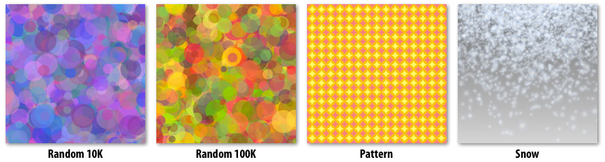
The directory /render of the assignment starter code contains an implementation of renderer that draws colored circles. Build the code, and run the render with the following command line: ./render rgb. You will see an image of three circles appear on screen (‘q’ closes the window). Now run the renderer with the command line ./render snow. You should see an animation of falling snow.
The assignment starter code contains two versions of the renderer: a sequential, single-threaded C++ reference implementation, implemented in refRenderer.cpp, and an incorrect parallel CUDA implementation in cudaRenderer.cu.
Renderer Overview
We encourage you to familiarize yourself with the structure of the renderer codebase by inspecting the reference implementation in refRenderer.cpp. The method setup is called prior to rendering the first frame. In your CUDA-accelerated renderer, this method will likely contain all your renderer initialization code (allocating buffers, etc). render is called each frame and is responsible for drawing all circles into the output image. The other main function of the renderer, advanceAnimation, is also invoked once per frame. It updates circle positions and velocities. You will not need to modify advanceAnimation in this assignment.
The renderer accepts an array of circles (3D position, velocity, radius, color) as input. The basic sequential algorithm for rendering each frame is:
 Clear image
 for each circle
     update position and velocity
 for each circle
     compute screen bounding box
     for all pixels in bounding box
         compute pixel center point
         if center point is within the circle
             compute color of circle at point
             blend contribution of circle into image for this pixel
Figure 2 illustrates the basic algorithm for computing circle-pixel coverage using point-in-circle tests. Notice that a circle contributes color to an output pixel only if the pixel’s center lies within the circle.
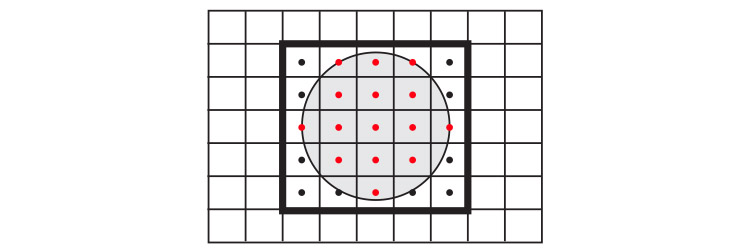
Figure 2 A simple algorithm for computing the contribution of a circle to the output image: All pixels within the circle’s bounding box are tested for coverage. For each pixel in the bounding box, the pixel is considered to be covered by the circle if its center point (black dots) is contained within the circle. Pixel centers that are inside the circle are colored red. The circle’s contribution to the image will be computed only for covered pixels.
CUDA Renderer
After familiarizing yourself with the circle rendering algorithm as implemented in the reference code, now study the CUDA implementation of the renderer provided in cudaRenderer.cu. You can run the CUDA implementation of the renderer using the —renderer cuda program option.
The provided CUDA implementation parallelizes computation across all input circles, assigning one circle to each CUDA thread. While this CUDA implementation is a complete implementation of the mathematics of a circle renderer, it contains several major errors that you will fix in this assignment. Specifically: the current implementation does not ensure image update is an atomic operation and it does not preserve the required order of image updates (the ordering requirement will be described below).
Renderer Requirements
Your parallel CUDA renderer implementation must maintain two invariants that are preserved trivially in the sequential implementation.
Atomicity: All image update operations must be atomic. The critical region includes reading the four 32-bit floating-point values (the pixel’s rgba color), blending the contribution of the current circle with the current image value, and then writing the pixel’s color back to memory.
Order: Your renderer must perform updates to an image pixel in circle input order. That is, if circle 1 and circle 2 both contribute to pixel P, any image updates to P due to circle 1 must be applied to the image before updates to P due to circle 2. As discussed in class, preserving the ordering requirement allows for correct rendering of transparent surfaces. (It has a number of other benefits for graphics systems.) A key observation is that the definition of order only specifies the order of updates to the same pixel. Thus, as shown in Figure 3, there are no ordering requirements between circles that do not contribute to the same pixel. These circles can be processed independently.
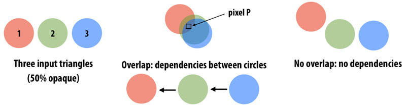
Figure 3. The contributions of circles 1, 2, and 3 must be applied to overlapped pixels in the order the circles are provided to the renderer.
Since the provided CUDA implementation does not satisfy these requirements, the result of not correctly respecting order can be seen by running the CUDA renderer implementation on the rgb and circles scenes. You will see horizontal streaks through the resulting images. These streaks will change with each frame.
What You Need To Do
Your job is to write the fastest, correct CUDA renderer implementation you can. You may take any approach you see fit, but your renderer must adhere to the atomicity and order requirements specified above. A solution that does not meet both requirements will be given no more than 2 points on the lab. We have already given you such a solution!
A good place to start would be to read through cudaRenderer.cu and convince yourself that it does not meet the correctness requirement. To visually see the effect of violation of above two requirements, compile the program with make. Then specify option ‘-r cuda -b 0:4 -f filename -s 768 rgb’ to dump the frame that was rendered. Compare this with ‘-b 0:4 -f filename -s 768 rgb’ which is the image generated by sequential code. This will generate ppm type of image files.
An example of sbatch file is the following.
 #!/bin/bash
 #SBATCH -J render           # job name
 #SBATCH -o render.oj expands to jobID)
 #SBATCH -n 1              # total number of mpi tasks requested
 #SBATCH -p gpudev     # queue (partition) — normal, development, etc.
 #SBATCH -t 01:30:00        # run time (hh:mm:ss) - 1.5 hours
 #SBATCH —mail-user=emailemail@gmail.com
 #SBATCH —mail-type=begin  # email me when the job starts
 #SBATCH —mail-type=end    # email me when the job finishes
 #SBATCH -A Fa16EE382N-20
 ./render -r cuda -b 0:4 -f rgbtest_cuda -s 768 rgb
Following are some of the options to ./render:
 -b  —bench START:END    Benchmark mode, do not create display. Time frames from START to END
 -c  —check              Runs both sequential and cuda versions and checks correctness of cuda version
 -f  —file  FILENAME     Dump frames in benchmark mode (FILENAME_xxxx.ppm)
 -r  —renderer WHICH     Select renderer: WHICH=ref or cuda
 -s  —size  INT          Make rendered image x pixels
 -?  —help               Prints information about switches mentioned here.
Checker code: To detect correctness of the program, render has a convenient —check option. This option runs the sequential version of the reference CPU renderer along with your CUDA renderer and then compares the resulting images to ensure correctness. The time taken by your CUDA renderer implementation is also printed.
We provide are total of five circle datasets you will be graded on. However, in order to receive full credit, your code must pass all of our test-benches. To check the correctness and performance score of your code, run ./checker.pl in the /render directory. If you run it on the starter code, the program will print a table like the following, along with the results of our entire test set:
 ------------
 Score table:
 ------------
 -------------------------------------------------------------------------
 | Scene Name      | Fast Time (Tf)  | Your Time (T)   | Score           |
 -------------------------------------------------------------------------
 | rgb             | 0.2615          | 137.9401 (F)    | 0               |
 | rand10k         | 10.1625         | 107.9893 (F)    | 0               |
 | rand100k        | 101.1337        | 1084.3314 (F)   | 0               |
 | pattern         | 0.9361          | 4.2878 (F)      | 0               |
 | snowsingle      | 59.4531         | 19.1290 (F)     | 0               |
 -------------------------------------------------------------------------
 |                                   | Total score:    | 0/65            |
 -------------------------------------------------------------------------
Note: on some runs, you may receive credit for some of these scenes, since the provided renderer’s runtime is non-deterministic. This doesn’t change the fact that the current CUDA renderer is incorrect.
“Fast time” is the performance of a good solution on your current machine (in the provided render_ref executable). “Your time” is the performance of your current CUDA renderer solution. Your grade will depend on the performance of your implementation compared to these reference implementations.
Along with your code, we would like you to hand in a clear, high-level description of how your implementation works as well as a brief description of how you arrived at this solution. Specifically address approaches you tried along the way, and how you went about determining how to optimize your code (For example, what measurements did you perform to guide your optimization efforts?).
Aspects of your work that you should mention in the write-up include:
- Include both partners names and UT EIDs at the top of your write-up.
- Replicate the score table generated for your solution and specify which machine you ran your code on.
- Describe how you decomposed the problem and how you assigned work to CUDA thread blocks and threads (and maybe even warps).
- Describe where synchronization occurs in your solution.
- What, if any, steps did you take to reduce communication requirements (e.g., synchronization or main memory bandwidth requirements)?
- Briefly describe how you arrived at your final solution. What other approaches did you try along the way. What was wrong with them?
Grading Guidelines
- For solutions that achieve significantly greater performance than required, bonus points will be awarded.
- Part 3 is the most important part of the lab and you should put more effort on part 3.
We will grade using a 5-level scale (I expect the final class grades to be in the A — B range with more ‘A’s and ‘A-‘s than ‘B’s):
| 5 | Truly remarkable work |
| 4 | Exceeded expectations (specifically with regards to learning goals) |
| 3 | Met expectations |
| 2 | Did not meet all learning goals expected |
| 1 | Requires significant changes |
Assignment Tips and Hints
Below are a set of tips and hints compiled from previous years. Note that there are various ways to implement your renderer and not all hints may apply to your approach.
- To facilitate remote development and benchmarking, we have created a —benchmark option to the render program. This mode does not open a display, and instead runs the renderer for the specified number of frames.
- When in benchmark mode, the —file option sets the base file name for PPM images created at each frame. Created files are basename xxxx.ppm. No PPM files are created if the —file option is not used.
- There are two potential axes of parallelism in this assignment. One axis is parallelism across pixels another is parallelism across circles (provided the ordering requirement is respected for overlapping circles).
- The prefix-sum operation provided in exclusiveScan.cu_inl may be valuable to you on this assignment (not all solutions may choose to use it). See the simple description of a prefix-sum here. We have provided an implementation of an exclusive prefix-sum on a power-of-two-sized array in shared memory. The provided code does not work on non-power-of-two inputs. IT ALSO REQUIRES THAT THE NUMBER OF THREADS IN THE THREAD BLOCK BE THE SIZE OF THE ARRAY.
- You are allowed to use the Thrust library in your implementation if you so choose. Thrust is not necessary to achieve the performance of the optimized CUDA reference implementations.
- Is there data reuse in the renderer? What can be done to exploit this reuse?
- The circle-intersects-box tests provided to you in circleBoxTest.cu_inl are your friend.
- How will you ensure atomicity of image update since there is no CUDA language primitive that performs the logic of the image update operation atomically? Constructing a lock out of global memory atomic operations is one solution, but keep in mind that even if your image update is atomic, the updates must be performed in the required order. We suggest that you think about ensuring order in your parallel solution first, and only then consider the atomicity problem (if it still exists at all) in your solution.
- If you are having difficulty debugging your CUDA code, you can use printf directly from device code if you use a sufficiently new GPU and CUDA library: see this brief guide on how to print from CUDA.
- If you find yourself with free time, have fun making your own scenes!
Hand-in Instructions
- Part 1,2 : Compress your working starter directory. The file name should be part12.tgz. Submit the file on canvas. Also submit the PDF report on Gradescope.
- Part 3 : Same as part 1,2 (file name: part3.tgz include all three directories) on canvas and write-up on Gradescope.


